Cooking with Snowflake

The Snowflake community is rife with information dumps on how to optimize expensive queries. We know because we combed through a ton of them. What we present here are three tactical ways in which we’ve done this at Toplyne.

Introduction

Toplyne’s business involves extracting real-time insights from real-time data. This data is currently sourced from our customers' Product Analytics, CRM, and payments system.

CRM and payment data volumes are mostly manageable. A product will have a limited set of paying customers and marginally more who are tracked in a CRM. However, product analytics data is much higher in volume.

Toplyne’s POC (proof-of-concept) and MVP (minimum viable product) were built on product analytics data. We knew right from the beginning we needed to use a Data Warehousing solution to handle the data. The solution had to pass two clear requirements:

1. It should easily ingest a few 100 gigabytes of data.

2. It should offer a simple yet concise API to interact with this data.

We compared 3 solutions: BigQuery, Redshift & Snowflake.

Post-exploration, Snowflake was a clear choice. The simple reason is its SQL-based interface. SQL meant there was no cold start latency for our engineering ops. None of the engineers at Toplyne came from a DWH background, still, we found ourselves up to speed very quickly.

The process of interacting with customers’ product analytics data is simple as follows:

1. The product analytics data lands into Snowflake via a connector. (There are a lot of over-the-counter as well as native connectors for the same).

2. Login to Snowflake and use the in-built worksheets to write SQL. 🎉

This simple 2-step process means that we can get on top of the data that our customers share with us in no time.

In a short period, we cooked up two algorithms to transform the data we receive into a schema that can be trained by our data scientists. The first algorithm took care of transforming the product analytics events data. The second took care of identifying users' profile data. Additional feature engineering algorithms are then written on top of this data.

SQL is a fourth-generation language (4GL) that is relatively easier to learn. Combined with a worksheet-based interface that just requires you to have a browser tab - Snowflake; a scrappy startup could do a lot of data-heavy lifting with minimal setup effort.

We wrote a few SQLs in the worksheet to transform the data and then our data scientists could just SELECT * the data and write their ML training programs.

Over time the entire above-mentioned process has scaled up significantly. The scaling up has happened in the following aspects:

1. We have multiple customers, each of whom has their product analytics data in multiple platforms viz., Amplitude, Mixpanel, Segment, Clevertap, etc.

2. Our teams have written multiple algorithms to crunch the data along different axes.

3. We now integrate CRM as well as payment data. Further, these datasets have their own set of ETL algorithms.

4. We use Airflow to orchestrate enormous pipelines which have multiple stages.

Sample architecture diagram of our ETL flow. Snowflake sits at the heart of this system.

1. Sync source data into Snowflake.

2. Use Apache Airflow for ETL orchestration.

3. Land the transformed data into Snowflake.

4. DS/ML/Analysts/Product consumes data from Snowflake for their flows.

Over the months, there have been multiple changes and major rewrites of different components of the system with Snowflake being the only constant.

As we have run and maintained a system, we would like to present a few ideas around query optimization in Snowflake. We have a super simple technique that has allowed us to extract a lot of performance from the system with minor tweaks in your existing queries.

Query optimization

We run a multi-tenant system wherein a single Snowflake instance is responsible for the ETL of a lot of customer data. ETL is orchestrated by Airflow.

We create a warehouse per customer and run all the ETL & feature engineering on that warehouse. There are 100s of SQL queries that are fired against a warehouse in sequence and/or in parallel during the entire ETL run for the customer. One run can last for an hour and there can be multiple runs for the customer in a day.

Essentially, one warehouse size runs all expensive as well as cheap queries. So our objective is to keep warehouse size at a minimum. We define minimums by defining SLAs for different ETL runs. Then we modify the warehouse size so that ETL SLAs can be met at that size. Like any engineering org, we want to keep the warehouse size at a bare minimum given the SLA.

We have dashboards where we monitor query patterns of the most expensive queries. These dashboards are at different levels of granularity. We monitor these dashboards constantly and keep tweaking the queries. Over time we have identified a few patterns in expensive queries and have come up with a playbook on how to minimize the run time of these queries. We’ll present 3 case studies outlining the problem statement for the query, how it was originally written, what was the bottleneck in that query and what was the optimal solution for the same.

Window queries

Scenario

We track users' profile information from product analytics data. Product Analytics systems save multiple data points about their users, e.g., location, device, subscription status, etc. Some data points change frequently while others do not so much. Given the nature of these data, the information is represented as an append-only log in a database.

One of our feature engineering requirements is to capture the users’ latest profile info as of the ETL run.

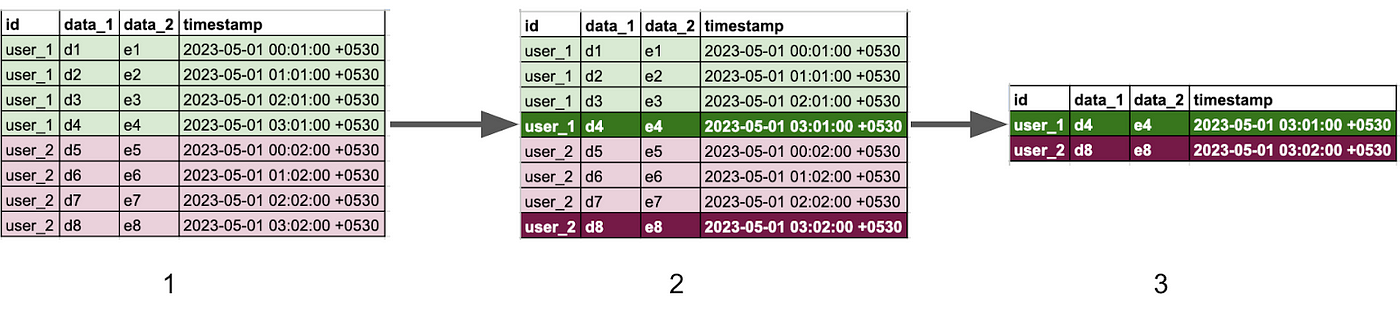
The above diagram gives a flowchart of the ETL.

1 is the raw_data from product analytics, 2 is the algorithm that we want to apply & 3 is the final result of the ETL.

The SQL query that we have is this:

select
    *
from
    tbl
qualify
    row_number() over (partition by id order by timestamp desc) = 1

Bottleneck

This query is pretty simple to come up with and works great in Snowflake. However, the window function in this query is a bottleneck.

Here’s how the query works:

1. create as many logical buckets as there are user_ids

2. sort data in every bucket in descending order

3. assign row_numbers to the arranged data

4. qualify the first entry in the bucket

5. discard the remaining data.

Based on the above explanation, we can see that as the data in the table increases, the number of buckets and the bucket sizes both will increase. Since we are dealing with an append-only dataset, we should be prepared for this eventuality. In Snowflake, you’ll notice the size increase trend as Byte Spillage in your query profiler.

Further, we need to understand that based on business requirements, it is expected for the number of buckets to increase, but as engineers, we can still keep the size of an individual bucket to a minimum.

Optimal solution

We’ll come up with a technique to keep the entries being bucketed to a minimum by using CTEs & an aggregate function.

with
prune_condition as (
    select id, max(timestamp) as prune_column from tbl group by id
),
pruned_data as (
    select * from tbl left join prune_condition using (id)
)
select
    * exclude prune_column
from
    pruned_data
where
    timestamp >= prune_column
qualify
    row_number() over (partition by id order by timestamp desc) = 1

We convert our descending sort expression in-the-window query clause to the max() function and then join that to our source data to obtain a filter. By using this filter, we ensure that the data that would have been discarded by the qualify clause anyways would never be bucketed in the first place. This reduces the work performed by the window query drastically. Also, the additional cost of using an aggregate function is massively offset by the reduction, so the overall query becomes performant.

Pivot queries

Scenario

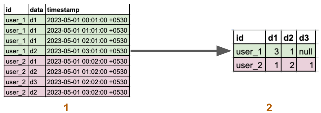
We use a feature on event data that requires getting a per-user per-event count.

To obtain this data, we perform a group by query and then transpose this data to organize it into columns as shown in the image below.

1 is the raw data & 2 is the output after the transformation.

The SQL query that we have is this:

select * from (
    select id, id as users, data from tbl
) pivot(
    count(users)
    for data in (‘d1’, ‘d2’, ‘d3’)
)

Bottleneck

Although the sample shows a pivot along 3 elements, our production use case generally functions on around a million users for approximately 1000 events.

The pivot function on this query is the slowest step of the query. So we want to replace this logic with a manual pivot query. We generate this query by using a combination of Group By clause & Filter clause.

Optimal solution 1

select 
    id,
    sum(iff(data = ‘d1’, 1, 0)) as “‘d1’”,
    sum(iff(data = ‘d2’, 1, 0)) as “‘d2’”,
    sum(iff(data = ‘d3’, 1, 0)) as “‘d3’”
from
    tbl
group by id

This query improved performance significantly.

We then reduced the warehouse size to see if the query remains equally performant. We observed that the query slowed down significantly and byte spillage was significant. However, an advantage of byte spillage is that we have more room for improvement in the reduced warehouse size.

Optimal Solution 2

We rewrote this query as per the Map-Reduce framework and observed a significant improvement in runtime.

The objective is to perform the above operation on a smaller set of events at a time and join all the data together in one go as follows:

create temporary batch_1 as (
    select
        id,
        sum(iff(data = ‘d1’, 1, 0)) as “‘d1’”
    from
        tbl
    group by id
);

create temporary batch_2 as (
    select
        id,
        sum(iff(data = ‘d2’, 1, 0)) as “‘d2’”,
        sum(iff(data = ‘d3’, 1, 0)) as “‘d3’”
    from
        tbl
    group by id
);

create final_table as (
    select * from batch_1 full outer join batch_2 using(id)
);

Our production system will break up 1000 events into 10 chunks of 100 events each. This query speeds up significantly as it reduces byte spillage to near 0.

Also, this optimization is quite intuitive to derive once we replace the Pivot function with Optimal Solution 1.

Aggregate queries

SQL spec defines a lot of aggregate functions and Snowflake does a great job at this. There is a massive repository of aggregate functions in Snowflake as well.

Different aggregate functions have varying runtimes and in our opinion, every aggregate function should be treated on its merit. A strategy for optimizing aggregate functions is to first identify aggregate functions to be a bottleneck and then motivate yourself that there might be an algorithmic solution to your problem statement.

We would like to share one case study with you where we identified a query in which a suboptimal aggregate function was chosen. We redid the algorithm for the solution using a simpler aggregate function thereby getting a far superior performance for the same result.

Scenario

We have a time series of events that are fired in the product analytics system. We need to answer 2 questions from this dataset for one of feature engineering.

Q1) Identify all data points that are mostly fired multiple times within a second

Q2) Identify data points that are mostly fired at least an hour apart

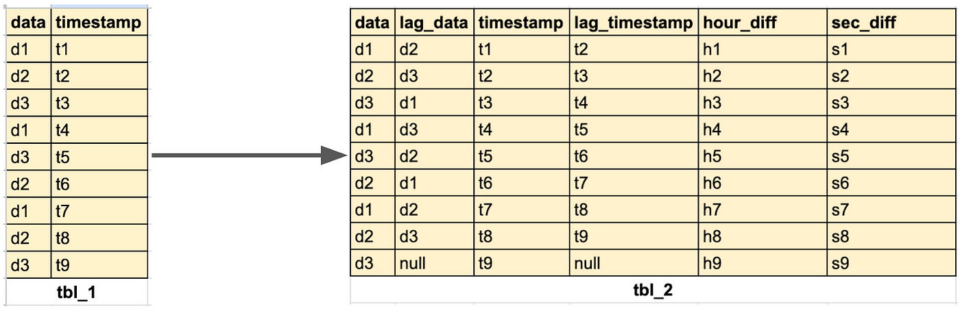
To answer these questions, we transform input data in tbl_1 to tbl_2 using a window query with the Snowflake lag function.

We then write the solution query using the median function as follows.

-- Q1)

select
    data
from
    tbl_2
group by data
having median(sec_diff) = 0;

-- Q2)

select
    data
from
    tbl_2
where
    data <> lag_data
group by data
having median(hour_diff) > 0;

Bottleneck

The median function is super slow.

We asked ChatGPT to suggest an optimal solution. It did come up with a solution to use a Percentile function, but that was equally slow and seemed synonymous with the Median function itself.

However, ChatGPT did a good job of explaining why it came up with that solution. We then came up with a solution by iterating & improving ChatGPT’s solution.

Optimal solution

We identified that for our requirement, we can just use count queries. For both Q1) & Q2), we want the majority of our events to have sec_diff & hour_diff respectively equal to & greater than 0.

-- Q1) after optimisation

select
    data,
    count(iff(sec_diff = 0, 1, null)) / count(*) as seccount
from
    tbl_2
group by data
having seccount >= 0.5

-- Q2) after optimisation

select
    data,
    count(iff(hour_diff > 0, 1, null)) / count(*) as hourcount
from
    tbl_2
group by data
having hourcount >= 0.5

TL;DR

Query optimization is a continuous process and requires investment in monitoring processes before any solutions can be derived.

It is also continuous as we don’t expect ourselves to sit down for a sprint and achieve it. We have to do it daily. We observe our systems constantly and then identify what optimizations require urgent analysis and what can be backlogged.

Snowflake provides multiple configuration parameters which can be tuned in conjunction to obtain performance. The Snowflake community regularly publishes tricks & techniques.

Among all this information overload, we need to focus and build a playbook & a repo of techniques that works for us and can be applied mindlessly.

These are the parameters that we use for our purpose:

1. Inspect every node in the query profiler

2. Do an input v/s output ratio for the node

   1. Try to bring down this ratio

   2. The output will remain constant given a problem statement

   3. Hence, try to reduce input to the aggregate node

3. Another way is to constantly measure the disk spillage. Reduce spillage whenever possible

   1. Larger warehouses have low spillage but also cost higher

   2. You get optimization only if you can reduce spillage in the same warehouse

      Working at Toplyne

      We’re looking for talented engineering interns to join our team. You can find and apply for relevant roles here.